Gail’s opens where London is already expensive. That isn’t a finding — it’s the business model. So the interesting question isn’t whether a bakery moves house prices. It’s the reverse: if a private-equity-backed chain is that careful about where it opens, how much does the resulting map tell you about London?
Quite a lot, as it turns out.
There is also a designed standalone version of this write-up, with the same content laid out properly.
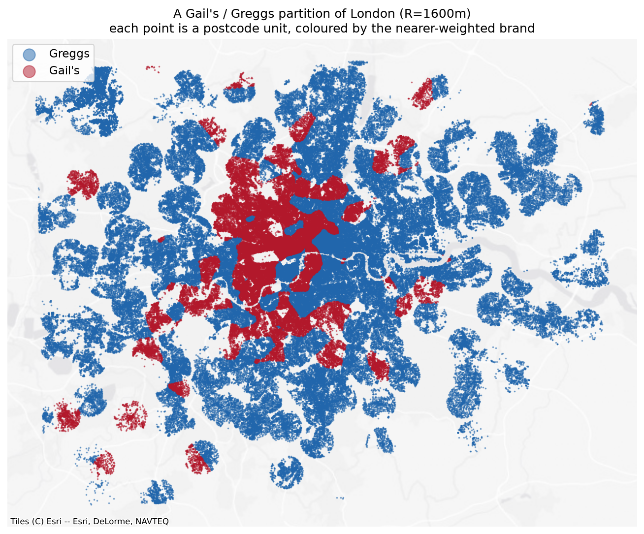
Each dot is one of 460,923 postcode units, coloured by which chain wins its distance-weighted accessibility score. Gail’s holds a contiguous central-and-west core plus scattered outposts — Richmond, Wimbledon, Blackheath, Chislehurst. Greggs holds everything else.
The question, and the trap in it
The obvious question — does a Gail’s nearby raise house prices? — is unanswerable with this data, and would be the wrong question even if it weren’t.
Gail’s sites deliberately into affluent, gentrifying, high-footfall catchments. Greggs sites onto high streets and transport nodes across the whole income distribution. Any positive coefficient is reverse causality by construction.
So the project asks something else: how good a measurement instrument is the bakery map? A proxy is supposed to read a pre-existing signal, not create one — which means the null result below isn’t a failed hypothesis. It’s a property the instrument needs to have.
Method
Shop locations come from OpenStreetMap merged with All The Places, reconciled into a slowly-changing dimension so openings and closures accumulate as an immutable event log rather than overwriting a table. The current estate is 136 Gail’s and 300 Greggs inside Greater London.
Prices are HM Land Registry Price Paid, category A, Greater London, 1995 to July 2026 — 3,724,260 transactions. Geography is the ONS Postcode Directory, which geocodes 99.94% of those sales to a British National Grid centroid and an LSOA. Retaining the 200,755 terminated postcodes is what makes the 1990s join work: the match rate never drops below 99.89% in any year back to 1995.
Accessibility uses a bisquare kernel with compact support, computed per postcode unit in EPSG:27700 so distances are straight metres:
Raw inverse-square was rejected — it diverges as d → 0, and a hard cap on top of it puts visible rings at radius R on the map. Two quantities come out of the kernel: a ratio measuring which chain dominates, and a level measuring how much bakery is nearby at all, which is essentially high-street-ness.
One thing worth flagging for anyone using this data: registration lag is far worse than the guidance suggests. The incomplete tail runs about nine months, not two. July 2026 holds 28% of a normal month’s sales. Rather than a fixed window, each month is scored against the median of months 12–24 back and carries a completeness ratio.
Result 1 — the causal reading is a null
Four specifications, each designed to break the one before. Standard errors clustered at LSOA; n = 2,388,494.
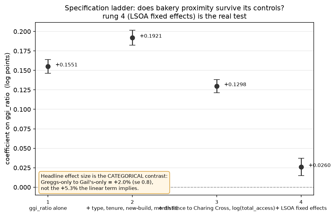
Rung 1 is the ratio alone (+0.155). Rung 2 adds property type, tenure, new-build and sale-month fixed effects. Rung 3 adds distance to Charing Cross and the level term. Rung 4 adds LSOA fixed effects — and 83% of the raw coefficient disappears.
What survives is real but small. And the linear form overstates it: 45% of sales sit at exactly −1 on the ratio (a Greggs-only catchment) and 6% at exactly +1, so a linear coefficient estimates a contrast between lumps while presenting as a slope. Entered as categories instead:
| Catchment | Coefficient | se | n |
|---|---|---|---|
| Greggs only | 0 (ref) | — | 1,074,473 |
| Mixed | +0.0102 | 0.0044 | 1,174,665 |
| Gail’s only | +0.0201 | 0.0082 | 139,356 |
+2.0% between a Greggs catchment and a Gail’s catchment, within one neighbourhood. The linear specification implies +5.3%, overstating it by a factor of 2.6.
The placebo
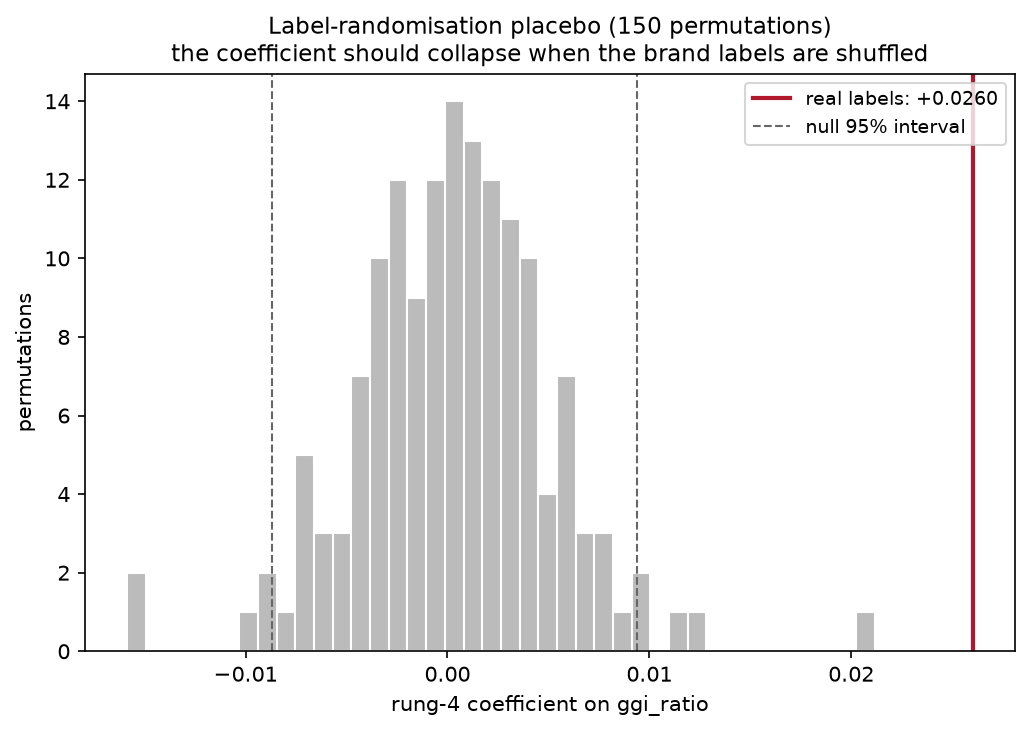
Shuffling the Gail’s/Greggs labels across the 436 real locations and re-running, 150 times. Null mean +0.0003, sd 0.0049, largest absolute draw 0.0211. The observed +0.0260 lies outside all 150 draws. The effect is real — it is simply small.
The pre-dating test
Take today’s bakery map and use it to predict sales from a decade ago, when most of the current Gail’s estate did not exist.
- 2015 sales: +0.0187 (se 0.0081)
- 2025 sales: +0.0258 (se 0.0080)
The difference is t = 0.63. Today’s Gail’s map predicts 2015 prices about as well as it predicts 2025 prices. Shops that opened after 2015 cannot have caused a price surface that already existed — which is exactly what a proxy reading a stable property of a place should look like.
Result 2 — what the ratio was hiding
A ratio forces Greggs to be Gail’s mirror image, so it can’t say whether Greggs proximity is good or bad on its own. Entering the two brands separately splits two effects that were cancelling:
| Term | Coefficient |
|---|---|
| Bakery density (either brand) | +0.0206 |
| Greggs accessibility | −0.0230 |
| Greggs present | −0.0396 |
| Gail’s accessibility | +0.0402 |
| Gail’s present | +0.2141 |
Two things fall out.
The mechanism you’d guess — “a Greggs means a working high street, and high streets are worth being near” — is half right. The high-street effect is real, but it lives in the density term. Greggs itself is negative, and holding density fixed makes it three times more so.
More interesting: Gail’s presence is a marker, not a dose. The presence term is five times the intensity term. One Gail’s tells you almost everything; five tell you barely more. That’s what you’d expect of a siting decision that is itself the signal.
Result 3 — how much of a neighbourhood model can two bakeries replace?
Hold property controls and sale-month fixed effects constant, then ask what share of the gap between no location information and 4,449 LSOA fixed effects each cheap location measure recovers. Out of sample, on a 477,492-sale holdout fitted from 1,911,001.
| Specification | Params | R² | Share |
|---|---|---|---|
| Base controls only — floor | 0 | 0.5698 | 0.0% |
| + LSOA fixed effects — ceiling | 4,449 | 0.8352 | 100.0% |
| + distance to nearest station | 1 | 0.5907 | 7.9% |
| + IMD 2019 rank | 1 | 0.6189 | 18.5% |
| + generic retail access (47,902 POIs) | 1 | 0.6518 | 30.9% |
| + distance to Charing Cross | 1 | 0.6720 | 38.5% |
| + bakery ratio and density | 2 | 0.6878 | 44.5% |
| + bakery terms, brands separate | 4 | 0.7095 | 52.6% |
| + IMD and distance | 2 | 0.7384 | 63.5% |
| + all four conventional | 4 | 0.7467 | 66.6% |
| + IMD, distance and bakery | 8 | 0.7638 | 73.1% |
| + all conventional and bakery | 10 | 0.7663 | 74.0% |
In-sample and out-of-sample shares agree to within 0.4 points on every row. The 4,449-parameter ceiling moves only 0.8359 → 0.8352, so it is barely overfitting at ~430 sales per LSOA.
The headline deflates, and then stops deflating. “44.5% of a 4,449-parameter model with two numbers” sounds remarkable until you notice distance to Charing Cross alone gets 38.5%. The number that survives scrutiny is the increment: adding the bakery terms on top of IMD and distance moves 63.5% → 73.1%, closing 27% of everything those two leave unexplained. That comparison has the obvious alternatives already in the model, so there’s nothing left to deflate it against.
Two bakery chains beat the official deprivation index by roughly 3× — 44.5% against 18.5%. That asymmetry cuts both ways, and it’s worth stating: IMD’s domains include income and employment deprivation, so it’s a survey-derived measure of socioeconomic status, partly built from the same forces that set prices. It is not a neutral competitor, and it is not built to predict prices. That makes its weak showing less surprising and the bakery index’s showing more so, since the latter uses nothing but coordinates.
Station distance is a genuine negative result. 7.9% alone, and +0.1 points on top of IMD and distance. London is dense enough with stations — median nearest 629 m — that the variable barely discriminates.
Is Gail’s vs Greggs actually the best pair?
Same machinery, six retail pairs, identical sample and parameter budget, ranked by increment over the full conventional stack.
| Pair | Outlets | Alone | Increment |
|---|---|---|---|
| Gail’s / Greggs | 105 / 225 | 51.0% | +6.7 |
| Waitrose / Iceland | 141 / 131 | 40.3% | +6.0 |
| Pret / Greggs | 316 / 225 | 36.4% | +3.1 |
| M&S Food / Poundland | 151 / 76 | 30.1% | +2.7 |
| Costa / Pret | 400 / 316 | 35.8% | +2.6 |
| Boots / Superdrug | 298 / 120 | 16.1% | +2.3 |
The obvious alternative explanation is resolution — a pair with 716 outlets has a finer-grained index than one with 330, regardless of how sharply the brands sort. The ranking already runs against that: Gail’s/Greggs has the second-smallest estate and ranks first, Costa/Pret has the largest and ranks fifth. Thinning Costa/Pret down to the incumbent’s exact counts costs it 0.2 points of increment. At identical outlet counts the gap is roughly threefold.
Two qualifications, both of which matter.
Waitrose/Iceland at +6.0 against +6.7 is not a commanding lead. On a different sample split I wouldn’t bet on the ordering between those two, and the gap to third place is far larger than the gap between first and second. The defensible claim is a clear top pair of two, with Gail’s/Greggs at its head.
More importantly, the field was selected on the dimension it is scored on. These six were chosen because they’re plausibly socially contrastive, and Gail’s/Greggs was chosen first precisely because the contrast is conspicuous. Winning a field selected for the property being ranked is weaker evidence than winning a random one.
What would have killed this, and what happened
Five tests designed to break the result:
- A broken pipeline. Label-shuffle placebo — the coefficient collapsed to noise on all 150 draws. Survived.
- A radial gradient in disguise. Added to distance-from-Charing-Cross, the bakery terms moved 38.5% → 60.1%. Survived.
- Redundant against conventional variables. Added on top of deprivation and distance, 63.5% → 73.1%. Survived.
- Merely finer-grained than its competitors. Aggregated to LSOA means, the increment grew rather than shrank. Survived.
- Just “how many shops are nearby”. Against all 47,902 OSM retail POIs, the bakery terms still added 16.9 points at matched parameter budget. Survived.
The only casualty was the causal reading — a claim the project never made.
Limitations
No floor area. Price Paid carries only property type, tenure and new-build. Floor area lives in EPC data, which isn’t ingested — so rungs 1 through 3 have weak property controls and their coefficients are inflated by an unknown amount. Rung 4 is the exception, since LSOA fixed effects compare houses within the same small neighbourhood.
The bandwidth question is undetermined, not answered.
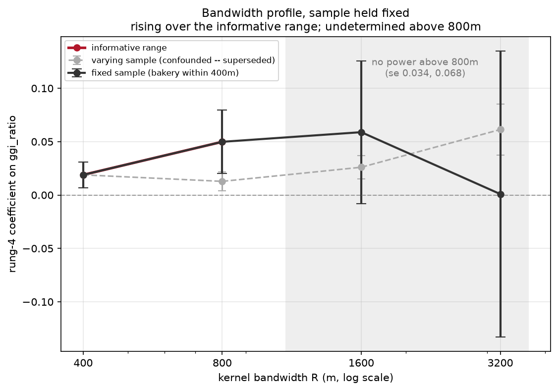
Across varying samples the coefficient rises fourfold with radius, which looks like evidence the index becomes a central-London gradient at wide bandwidths. It isn’t — that comparison is confounded by sample composition. But held to a fixed sample the standard errors run 0.006, 0.015, 0.034, 0.068, so only 400 m and 800 m carry information. Above 800 m the design has no power. Undetermined, not null.
Descriptive, not causal. Nothing here identifies a causal effect of anything on anything.
Current shops, historical sales. The index uses the 2026 estate against sales back to 1995. That anachronism is real, and the pre-dating test measures its consequence directly rather than apologising for it — the index working equally well in 2015 is the evidence for reverse causality, not a defect to be corrected.
Parameter budget matters. Against generic retail at one parameter the bakery terms add 25.5 points; at a matched four-parameter budget they add 16.9. The conclusion holds either way, but the magnitude is budget-dependent.
The index itself
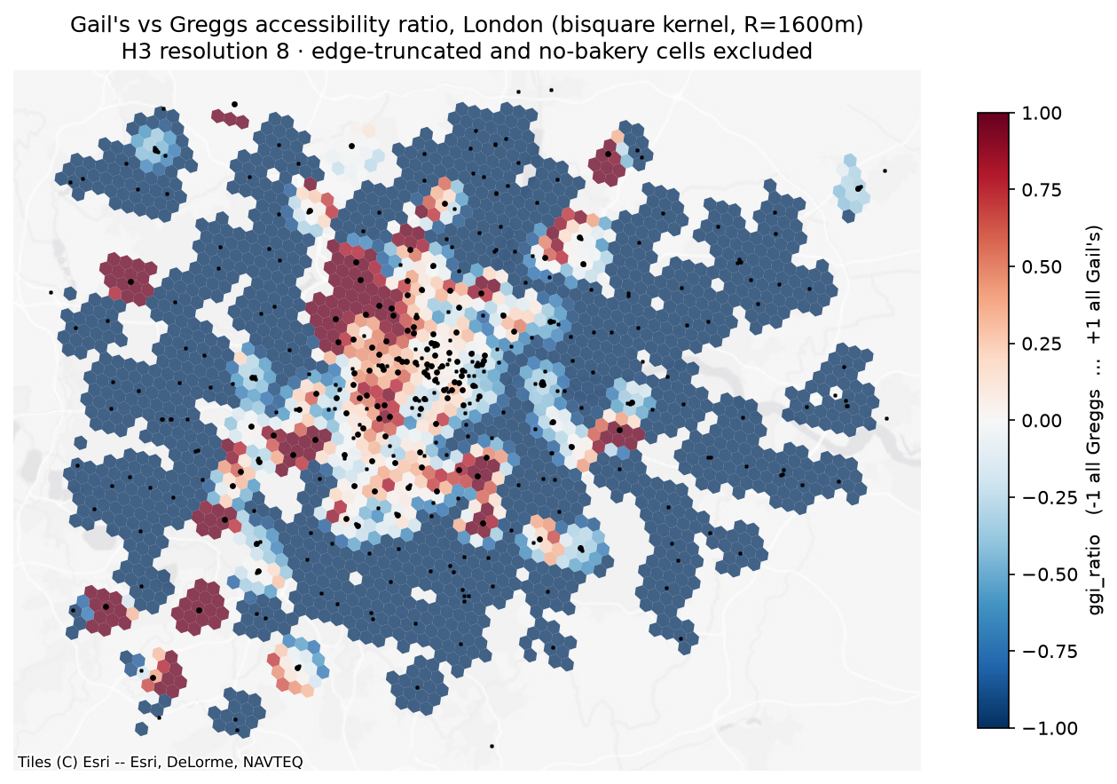
H3 resolution-8 cells coloured by the ratio; black dots are individual shops. The structure the regression works with is visible here — a red core with sharp boundaries, a deep-blue periphery, and a thin transitional band, which is why the ratio behaves closer to three categories than to a continuous scale.
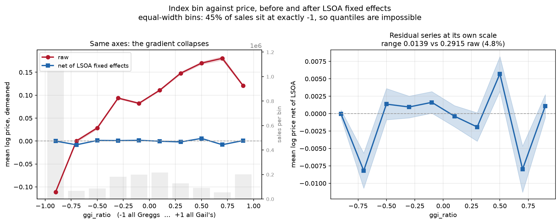
Mean log price by index bin, raw and after LSOA fixed effects are partialled out. The raw gradient spans 0.29 log points; net of neighbourhood, 4.8% of that survives, and non-monotonically. The flattening between the two series is the null in one picture.
Build notes
The pipeline is reproducible from a clean checkout and runs under a 512 MB DuckDB ceiling on an 8 GB machine — a constraint that shaped the design more than expected, and cost three out-of-memory kills before the Price Paid backfill was staged year-by-year and made resumable.
Things that turned out to matter more than the statistics:
- Content-hashed idempotent downloads, per-source watermarks, and add/change/delete upsert against the monthly Land Registry change file, which is not append-only.
- Entity resolution across sources — spatial matching at 50 m, stable-id matching taking precedence, and explicit split/merge rules for when one row is claimed by two observations.
- Alerting on match-rate drops rather than exceptions, because the failure mode that actually bites is a join quietly falling from 97% to 60%.
- Repudiable runs, since a bad run can commit and the event log is immutable.
Stack: Python 3.12, DuckDB, uv, pytest (139 tests), pyfixest, GeoPandas, matplotlib.
Sources: HM Land Registry Price Paid and ONS Postcode Directory (OGL v3); MHCLG Index of Multiple Deprivation 2019; OpenStreetMap via Overpass (ODbL); All The Places. Contains HM Land Registry data © Crown copyright and database right 2026. Contains OS data © Crown copyright and database right 2026. Contains Royal Mail data © Royal Mail copyright and database right 2026. Contains National Statistics data © Crown copyright and database right 2026.